TensorFlow 2.0 Tutorial 01: Basic Image Classification

TensorFlow 2 is now live! This tutorial walks you through the process of building a simple CIFAR-10 image classifier using deep learning. In this tutorial, we will:

• Define a model
• Set up a data pipeline
• Train the model
• Accelerate training speed with multiple GPUs
• Add callbacks for monitoring progress/updating learning schedules

The code in this tutorial is available here.

Defining a model

TensorFlow 2 uses Keras as its high-level API. Keras provides two ways to define a model: the Sequential API and functional API.

Defining a model using Keras' Sequential API

from tf.keras.models import Sequential
from tf.keras.layers import Conv2, MaxPooling2D, Flatten, Dense

model = Sequential([
    Conv2D(32, (3, 3), activation='relu', input_shape=(32, 32, 3)),
    MaxPooling2D(pool_size=(2, 2)),
    Flatten(),
    Dense(10, activation='softmax')
])

Defining the same model using Keras' functional API

from tf.keras.models import Model
from tf.keras.layers import Input, Conv2, MaxPooling2D, Flatten, Dense

inputs = Input(shape=(32, 32, 3))
x = Conv2D(32, (3, 3), activation='relu')(inputs)
x = MaxPooling2D(pool_size=(2, 2))(x)
x = Flatten()(x)
x = Dense(10, activation='softmax')(x)
model = Model(inputs=inputs, outputs=x)

Sequential vs. Functional APIs

The main difference between these APIs is that the Sequential API requires its first layer to be provided with input_shape, while the functional API requires its first layer to be tf.keras.layers.Input and needs to call the tf.keras.models.Model constructor at the end.

The Sequential API is more concise, while functional API is more flexible because it allows a model to be non-sequential. For example, to have the skip connection in ResNet. This tutorial adapts TensorFlow's official Keras implementation of ResNet, which uses the functional API.

input_shape = (32, 32, 3)
img_input = Input(shape=input_shape)
model = resnet_cifar_model.resnet56(img_input, classes=10)

Setting up a data pipeline

We've now defined a model. To train this model, we need a data pipeline to feed it labeled training data. A data pipeline performs the following tasks:

• Loading: Copying the dataset (e.g. images and labels) from storage into the program's memory.
• Preprocessing: transforming the dataset. For example, in image classification, we might resize, whiten, shuffle, or batch images.
• Feeding: shoveling examples from a dataset into a training loop.

Loading data from storage

First, we load CIFAR-10 from storage into numpy ndarrays:

(x, y), (x_test, y_test) = keras.datasets.cifar10.load_data()

Note that:

• The first time you call keras.datasets.cifar10.load_data, CIFAR-10 will be downloaded from the internet to ~/.keras/datasets/cifar-10-batches-py.tar.gz. Subsequent calls do not involve network.
• x represents 50,000 images with dimension 32 x 32 x 3 (width, height, and three RGB channels).
• y represents labels for these 50,000 images.

print(type(x), type(y))
(<type 'numpy.ndarray'>, <type 'numpy.ndarray'>)

print(x.shape, y.shape)
((50000, 32, 32, 3), (50000, 1))

In theory, we could simply feed these raw numpy.ndarray objects into a training loop and call this a data pipeline. However, to achieve higher model accuracy, we'll want to preprocess the data (i.e. perform certain transformations on it before usage). To do so, we leverage Tensorflow's Dataset class.

The tf.data.Dataset class

The TensorFlow Dataset class serves two main purposes:

• It acts as a container that holds training data.
• It can be used to perform alterations on elements of the training data.

We instantiate a tensorflow.data.Dataset object representing the CIFAR-10 dataset as follows:

# Load data from storage to memory.
(x, y), (x_test, y_test) = keras.datasets.cifar10.load_data()

# Instantiate the Dataset class.
train_dataset = tf.data.Dataset.from_tensor_slices((x, y))

During training, the CIFAR-10 training examples stored in train_dataset will be accessed via the take() iterator:

for image, label in train_dataset.take(1):
    (image.shape, label.shape)

As is, we perform no data preprocessing. Calling take() simply emits raw CIFAR-10 images; the first 20 images are as follows:

Data augmentation

Augmentation is often used to "inflate" training datasets, which can improve generalization performance.

Let's augment the CIFAR-10 dataset by performing the following steps on every image:

1. Pad the image with a black, four-pixel border.
2. Randomly crop a 32 x 32 region from the padded image.
3. Flip a coin to determine if the image should be horizontally flipped.

We achieve this by first defining a function that, given an image, performs the Steps 1-3 above:

def augmentation(x, y):
    x = tf.image.resize_with_crop_or_pad(
        x, HEIGHT + 8, WIDTH + 8)
    x = tf.image.random_crop(x, [HEIGHT, WIDTH, NUM_CHANNELS])
    x = tf.image.random_flip_left_right(x)
    return x, y

Next, we call the method map; this call returns a new Dataset object that contains the result of passing each image in CIFAR-10 into augmentation. This new object will emit transformed images in the original order:

train_dataset = train_dataset.map(augmentation)

These are the first 20 images after augmentation:

Note: Augmentation should only be applied to the training set; applying augmentation during inference would result in nondetermistic prediction and validation scores.

Shuffling

We randomly shuffle the dataset. TensorFlow Dataset has a shuffle method, which can be chained to our augmentation as follows:

train_dataset = (train_dataset
                 .map(augmentation)
                 .shuffle(buffer_size=50000))

For perfect shuffling, the buffer_size should be greater than or equal to the size of the dataset (in this case: 50,000); for large datasets, this isn't possible.

Below are 20 images from the Dataset after shuffling:

Normalization

It's common practice to normalize data. Here, define a function that linearly scales each image to have zero mean and unit variance:

def normalize(x, y):
  x = tf.image.per_image_standardization(x)
  return x, y

Next, we chain it with our augmentation and shuffling operations:

train_dataset = (train_dataset
                 .map(augmentation)
                 .shuffle(buffer_size=50000)
                 .map(normalize))

Batching

Finally, we batch the dataset. We set drop_remainder to True to remove enough training examples so that the training set's size is divisible by batch_size.

train_dataset = (train_dataset.map(augmentation)
                 .map(normalize)
                 .shuffle(50000)
                 .batch(128, drop_remainder=True)

We now have a complete data pipeline. Now we can start training.

Training the model

A Keras model needs to be compiled before training. Compilation essentially defines three things: the loss function, the optimizer and the metrics for evaluation:

model.compile(
          loss='sparse_categorical_crossentropy',
          optimizer=keras.optimizers.SGD(learning_rate=0.1, momentum=0.9),
          metrics=['accuracy'])

Notice we use sparse_categorical_crossentropy and sparse_categorical_accuracy here because each label is represented by a single integer (index of the class). One should use categorical_crossentropy and categorical_accuracy if a one-hot vector represents each label.

Keras uses the fit API to train a model. Optionally, one can test the model on a validation dataset at every validation_freq training epoch.

Notice we use the test dataset for validation only because CIFAR-10 does not natively provide a validation set. Validation of the model should be conducted on a set of data split from the training set.

model.fit(train_dataset,
          epochs=60,
          validation_data=test_dataset,
          validation_freq=1)

Notice in this example, the fit function takes TensorFlow Dataset objects (train_dataset and test_dataset). As previously mentioned, it can also take numpy ndarrays as the input. The downside of using arrays is the lack of flexibility to apply transformations on the dataset.

model.fit(x, y,
          batch_size=128, epochs=5, shuffle=True,
          validation_data=(x_test, y_test))

To evaluate the model, call the evaluate method with the test dataset:

model.evaluate(test_loader)

Multi-GPU

So far, we have shown how to use TensorFlow's Dataset API to create a data pipeline, and how to use the Keras API to define the model and conduct the training and evaluation. The next step is to make the code run with multiple GPUs.

In fact, Tensorflow 2 has made it very easy to convert your single-GPU implementation to run with multiple GPUs. All you need to do is define a distribute strategy and create the model under the strategy's scope:

mirrored_strategy = tf.distribute.MirroredStrategy()
with mirrored_strategy.scope():
    model = resnet.resnet56(classes=NUM_CLASSES)
    model.compile(
            optimizer=keras.optimizers.SGD(learning_rate=0.1, momentum=0.9),
              loss='sparse_categorical_crossentropy',
              metrics=['accuracy'])  

We use MirroredStrategy here, which supports synchronous distributed training on multiple GPUs on one machine. By default, it uses NVIDIA NCCL as the multi-gpu all-reduce implementation.

Note that you'll want to scale the batch size with the data pipeline's batch method based on the number of GPUs that you're using.

train_loader = train_loader.map(preprocess).shuffle(50000).batch(BS_PER_GPU*NUM_GPUS)
test_loader = test_loader.map(preprocess).batch(BS_PER_GPU*NUM_GPUS)

Adding callbacks

Often we need to perform custom operations during training. For example, you might want to log statistics during the training for debugging or optimization purposes; implement a learning rate schedule to improve the efficiency of training; or save visual snapshots of filter banks as they converge. In TensorFlow 2, you can use the callback feature to implement customized events during training.

Tensorboard

TensorBoard is mainly used to log and visualize information during training. It is handy for examining the performance of the model. Tensorboard support is provided via the tensorflow.keras.callbacks.TensorBoard callback function:

from tensorflow.keras.callbacks import TensorBoard

log_dir="logs/fit/" + datetime.datetime.now().strftime("%Y%m%d-%H%M%S")

tensorboard_callback = TensorBoard(
    log_dir=log_dir, update_freq='batch', histogram_freq=1)
  
model.fit(...,
          callbacks=[tensorboard_callback])

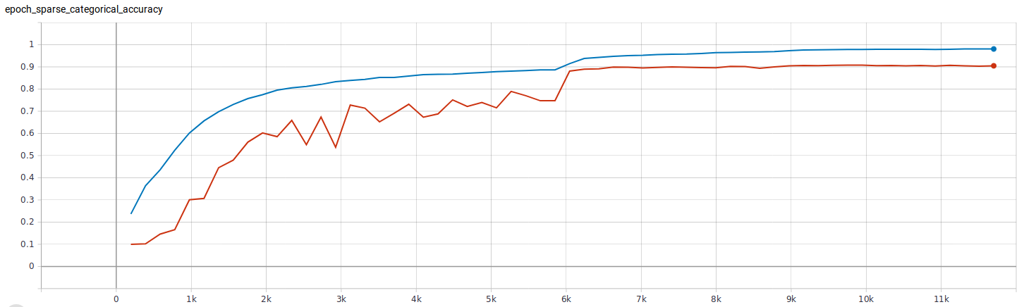
In the above example, we first create a TensorBoard callback that record data for each training step (via update_freq=batch), then attach this callback to the fit function. TensorFlow will generate tfevents files, which can be visualized with TensorBoard. For example, this is the visualization of classification accuracy during the training (blue is the training accuracy, red is the validation accuracy):

Learning Rate Schedule

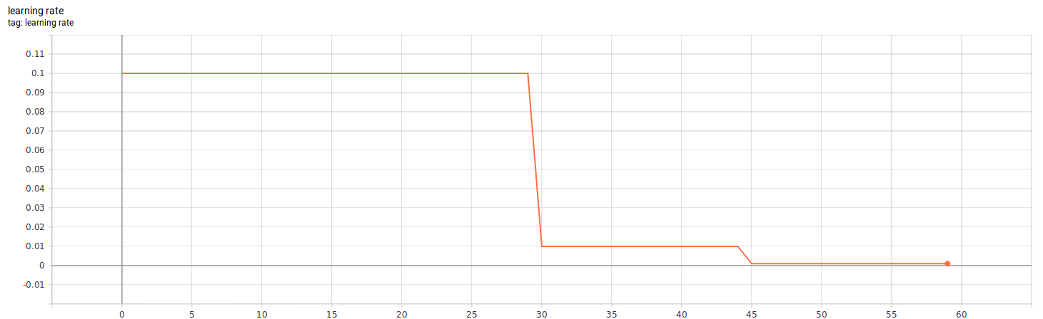
Often, we would like to have fine control of learning rate as the training progresses. A custom learning rate schedule can be implemented as callback functions. Here, we create a customized schedule function that decreases the learning rate using a step function (at 30th epoch and 45th epoch). This schedule is converted to a keras.callbacks.LearningRateScheduler and attached to the fit function.

from tensorflow.keras.callbacks import LearningRateScheduler

BASE_LEARNING_RATE = 0.1
LR_SCHEDULE = [(0.1, 30), (0.01, 45)]

def schedule(epoch):
  initial_learning_rate = BASE_LEARNING_RATE * BS_PER_GPU / 128
  learning_rate = initial_learning_rate
  for mult, start_epoch in LR_SCHEDULE:
    if epoch >= start_epoch:
      learning_rate = initial_learning_rate * mult
    else:
      break
  tf.summary.scalar('learning rate', data=learning_rate, step=epoch)
  return learning_rate
  
lr_schedule_callback = LearningRateScheduler(schedule)

model.fit(...,
          callbacks=[..., lr_schedule_callback])

These are the statistics of the customized learning rate during a 60-epochs training:

Summary

This tutorial explains the basic of TensorFlow 2.0 with image classification as an example. We covered:

• Data pipeline with TensorFlow 2's dataset API
• Train, evaluation, save and restore models with Keras (TensorFlow 2's official high-level API)
• Multiple-GPU with distributed strategy
• Customized training with callbacks

Below is the full code of this tutorial. You can also reproduce our tutorials on TensorFlow 2.0 using this Tensorflow 2.0 Tutorial repo.

import datetime

import tensorflow as tf
from tensorflow import keras
from tensorflow.keras.callbacks import TensorBoard, LearningRateScheduler

import resnet


NUM_GPUS = 2
BS_PER_GPU = 128
NUM_EPOCHS = 60

HEIGHT = 32
WIDTH = 32
NUM_CHANNELS = 3
NUM_CLASSES = 10
NUM_TRAIN_SAMPLES = 50000

BASE_LEARNING_RATE = 0.1
LR_SCHEDULE = [(0.1, 30), (0.01, 45)]


def preprocess(x, y):
  x = tf.image.per_image_standardization(x)
  return x, y


def augmentation(x, y):
    x = tf.image.resize_with_crop_or_pad(
        x, HEIGHT + 8, WIDTH + 8)
    x = tf.image.random_crop(x, [HEIGHT, WIDTH, NUM_CHANNELS])
    x = tf.image.random_flip_left_right(x)
    return x, y	


def schedule(epoch):
  initial_learning_rate = BASE_LEARNING_RATE * BS_PER_GPU / 128
  learning_rate = initial_learning_rate
  for mult, start_epoch in LR_SCHEDULE:
    if epoch >= start_epoch:
      learning_rate = initial_learning_rate * mult
    else:
      break
  tf.summary.scalar('learning rate', data=learning_rate, step=epoch)
  return learning_rate


(x,y), (x_test, y_test) = keras.datasets.cifar10.load_data()

train_dataset = tf.data.Dataset.from_tensor_slices((x,y))
test_dataset = tf.data.Dataset.from_tensor_slices((x_test, y_test))

tf.random.set_seed(22)
train_dataset = train_dataset.map(augmentation).map(preprocess).shuffle(NUM_TRAIN_SAMPLES).batch(BS_PER_GPU * NUM_GPUS, drop_remainder=True)
test_dataset = test_dataset.map(preprocess).batch(BS_PER_GPU * NUM_GPUS, drop_remainder=True)

input_shape = (32, 32, 3)
img_input = tf.keras.layers.Input(shape=input_shape)
opt = keras.optimizers.SGD(learning_rate=0.1, momentum=0.9)

if NUM_GPUS == 1:
    model = resnet.resnet56(img_input=img_input, classes=NUM_CLASSES)
    model.compile(
              optimizer=opt,
              loss='sparse_categorical_crossentropy',
              metrics=['sparse_categorical_accuracy'])
else:
    mirrored_strategy = tf.distribute.MirroredStrategy()
    with mirrored_strategy.scope():
      model = resnet.resnet56(img_input=img_input, classes=NUM_CLASSES)
      model.compile(
                optimizer=opt,
                loss='sparse_categorical_crossentropy',
                metrics=['sparse_categorical_accuracy'])  

log_dir="logs/fit/" + datetime.datetime.now().strftime("%Y%m%d-%H%M%S")
file_writer = tf.summary.create_file_writer(log_dir + "/metrics")
file_writer.set_as_default()
tensorboard_callback = TensorBoard(
  log_dir=log_dir,
  update_freq='batch',
  histogram_freq=1)

lr_schedule_callback = LearningRateScheduler(schedule)

model.fit(train_dataset,
          epochs=NUM_EPOCHS,
          validation_data=test_dataset,
          validation_freq=1,
          callbacks=[tensorboard_callback, lr_schedule_callback])
model.evaluate(test_dataset)

model.save('model.h5')

new_model = keras.models.load_model('model.h5')
 
new_model.evaluate(test_dataset)