Tracking system resource (GPU, CPU, etc.) utilization during training with the Weights & Biases Dashboard

One of the most asked questions we get at Lambda Labs is, “how do I track resource utilization for deep learning jobs?” Resource utilization tracking can help machine learning engineers improve both their software pipeline and model performance.

I recently came across a tool called "Weights and Biases" (wandb). If you, like me, used to track training jobs by a handful of different tools (nvidia-smi, htop, TensorBoard, etc.), then wandb is an excellent alternative. I have been playing around with it for a week, and now entirely rely on it for bookkeeping my deep learning experiments. In essence, wandb offers a centralized place to track not only the model-related information (weights, gradients, losses, etc.) but also the entire system utilization (GPU, CPU, Networking, IO, etc.). Plus, it is almost effortless to use – all you need to do is adding a few lines of code into your TensorFlow or PyTorch scripts.

The rest of this blog describes how to use wandb to profile TensorFlow training jobs. Our main goal is to help you understand training efficiency with the help of wandb's resource utilization graphing functionality. In particular we will:

• Understand the system diagrams in the wandb dashboard
• Use the diagrams to analyze your training efficiency

We will also cover the basic installation of wandb and how to integrate wandb with your TensorFlow code.

Installation

Installing wandb is acturally very easy. First, you need a computer that can run Deep Learning frameworks such as TensorFlow or Pytorch. My first wandb experiment ran with the CPU version of TensorFlow on a laptop. However, nowadays most people run deep learning experiments with a GPU, in which case it is necessary to first install NVIDIA driver and CUDA.

The wandb team recommend using Python virtual environment, which is what we will do in this tutorial. Below are the commands to create a clean python virtual environment on Linux, install TensorFlow and wandb. We provide commands for installing both the CPU and the GPU versions of TensorFlow-CPU and TensorFlow. The rest of the tutorial will use the GPU version and run experiments on a dual GPU Lambda workstation.

# Create python virtual environment
pip install virtualenv
virtualenv myenv
. myenv/bin/activate

# Install TensorFlow CPU
pip install tensorflow==1.13.1

# Install TensorFlow with GPU support
pip install tensorflow-gpu==1.13.1

# Install wandb
pip install wandb

TensorFlow Integration

To use wandb with TensorFlow, simply add a couple of lines of code to the main training script. Let's first clone the official TensorFlow benchmark Repo:

# Clone TensorFlow benchmark Repo
git clone https://github.com/tensorflow/benchmarks.git
cd benchmarks/scripts/tf_cnn_benchmarks
git checkout cnn_tf_v1.13_compatible

Then add the following lines to the benchmark_cnn.py file, at the end of the imports.

import wandb as wb
wb.init(sync_tensorboard=True)

Notice these lines should be added to the main script. In the case of TensorFlow, you should look for the script that creates the training loop and calls sess.run. Integrating wandb with other deep learning frameworks, such as PyTorch and Keras, is just as straightforward. Please refer to the official wandb documentation for details.

Before running your experiment, log in your wandb account. Simply run the following line in your command-line interface:

wandb login

You will be asked to log in from a web interface. Notice wandb is currently (August 2019) free for individual users.

That's it. Now you can run the script as usual, and wandb will dynamically update the logs in the web interface. For example, here is the command of training AlexNet on two GPUs:

python tf_cnn_benchmarks.py --data_format=NCHW --batch_size=4 --model=alexnet --optimizer=momentum --variable_update=replicated --gradient_repacking=8 --num_gpus=2 --num_batches=10000 --weight_decay=1e-4

wandb's web interface displays a dashboard with all the excuted experiments. Here are the ones that I ran for this blog:

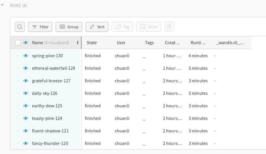
Dashboard

Dashboard is the centralized place to sift through the experiments. Let's click on the experiment "fancy-thunder-120" and see what has been logged there.

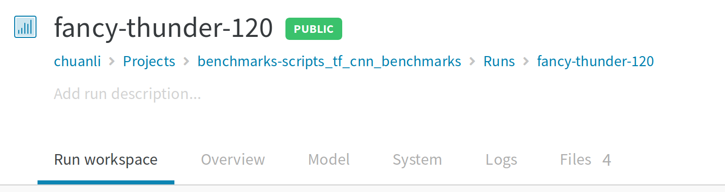
As you can see, wandb groups information into different sections. We will discuss the Overview, Logs, and the System sections. In particular, how to get insights into the training efficiency through the System section.

Overview

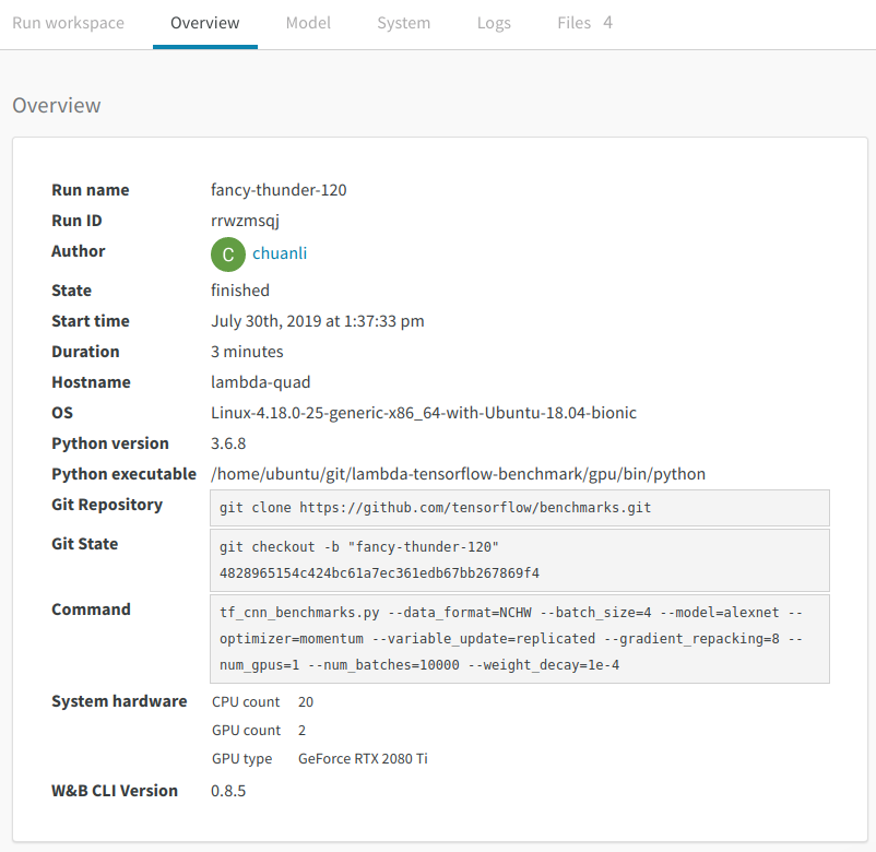
The information in the overview section is pretty intuitive and self-explanatory. However, the Git Repository field and the Git State field are worthy of special mention. You can run the checkout command in the Git State field to pin down the exact code for reproducing the experiment. Under the hood, wandb tracks all the changes you made to the original repo, and save the "diff" files in a local directory. In this way, you can easily switch between different versions of the code without manually pushing the change to the remote repo.

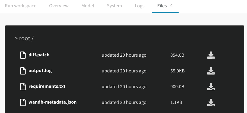
But what happens if you accidentally delete the local files? No problem, wandb automatically stores these files on their server for every finished experiment, so you can download them whenever is necessary. These backup files can be found in the "Files" section of the dashboard.

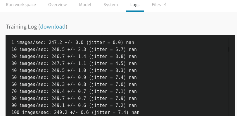
Logs

The logs section shows the console output during the experiment. This is useful for debugging the performance of the model.

Systems

To me, the system section is where wandb really shines and separates itself from other options such as TensorBoard. It is a centralized place to track system utilization during the experiment. There are in total of 8 graphs displayed in this section. These graphs give you insight into the training bottleneck and possible ways to uplift it. For example, below are the diagrams of the experiment "fancy-thunder-120":

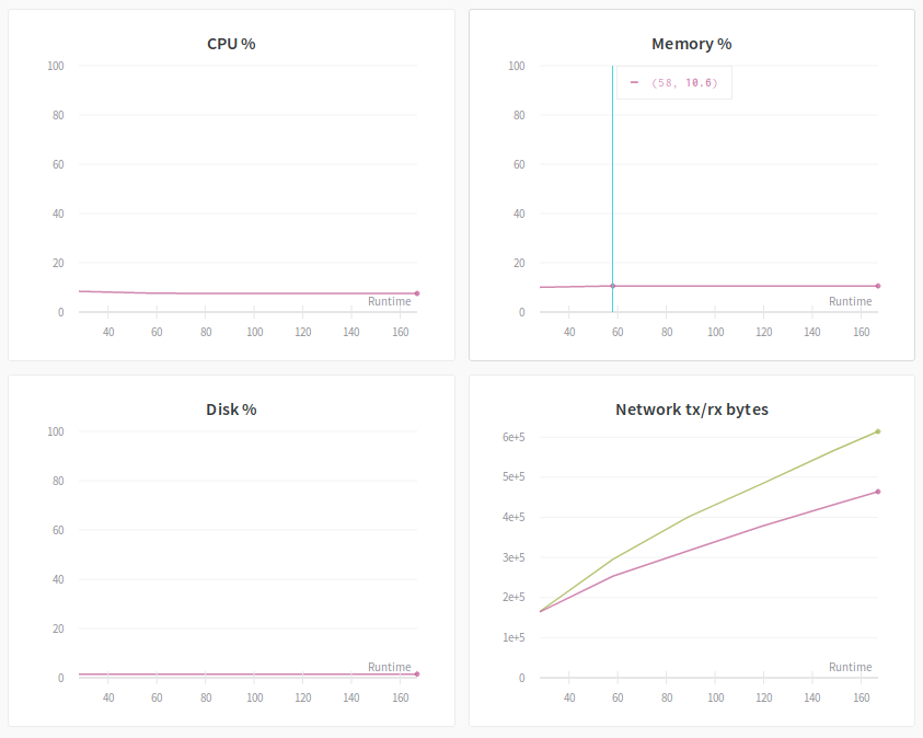
Let's firt clarify the hyper-parameters for the experiment: we use synthetic data to train an AlexNet with batch size=4. There are two GPUs in the system, but we only enable one for the experiment by prefixing the training command with CUDA_VISIBLE_DEVICES=0.

Now, let's see what the above graphs do:

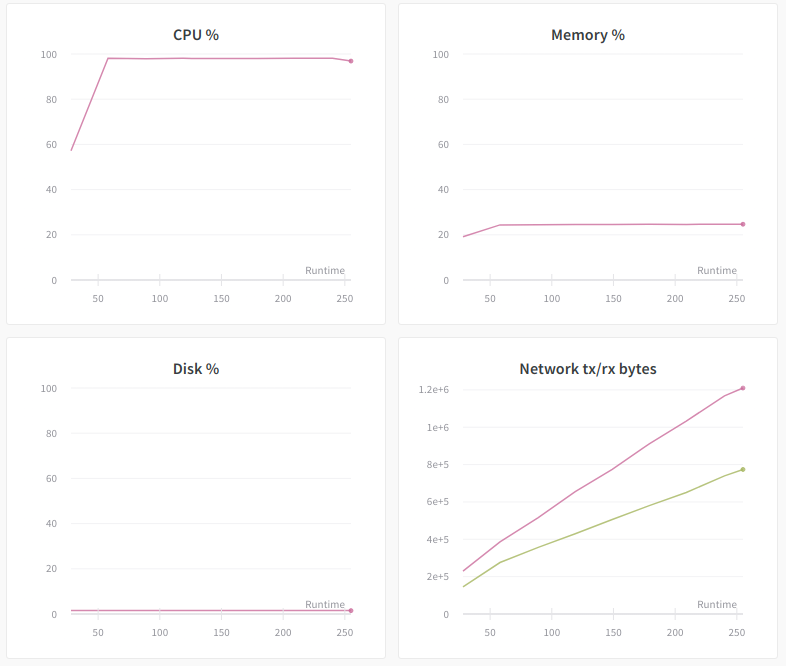
• CPU %: This graph shows the CPU utilization during the training. In this example, there is little workload on the CPU. This is because synthetic data are stored in the GPU memory. In the meantime, no image augmentation is used.
• Memory %: This graph shows the system memory utilization during the training. In this case, there is little system memory used because the data are directly hosted on the GPU memory.
• Disk %: This graph shows the disk utilization. Once again, no much happened here because there is no reading data from the disk.
• Network tx/rx bytes: Records the network traffic. Not much here since only a single machine is used.
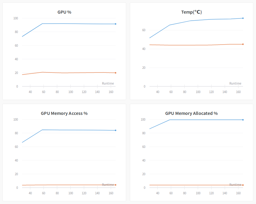
• GPU %: This graph is probably the most important one. It tracks the percent of the time over the past sample period during which one or more kernels was executing on the GPU. Basically, you want this to be close to 100%, which means GPU is busy all the time doing data crunching. The above diagram has two curves. This is because there are two GPUs and only of them (blue) is used for the experiment. The Blue GPU is about 90% busy, which means it is not too bad but still has some room for improvement. The reason for this suboptimal utilization is due to the small batch size (4) we used in this experiment. The GPU fetches a small amount of data from its memory very often, and can not saturate the memory bus nor the CUDA cores. Later we will see it is possible to bump up this number by merely increasing the batch size.
• Temp (C): This is also a very important metric. It tracks the temperature of the GPUs during the experiment. You don't want your GPU to become overheat, which does not only slow down the training but also damages the hardware. In the above figure, you can see the temperature difference between a busy GPU (blue, around 73 C) and an idle GPU (orange, around 45 C).
• GPU Memory Access %: This is an interesting one. It measures the percent of the time over the past sample period during which GPU memory was being read or written. We should keep this percent low because you want GPU to spend most of the time on computing instead of fetching data from its memory. In the above figure, the busy GPU has around 85% uptime accessing memory. This is very high and caused some performance problem. One way to lower the percent here is to increase the batch size, so data fetching becomes more efficient.
• GPU Memory Allocated %: This indicates the percent of the GPU memory that has been used. We see 100% here mainly due to the fact TensorFlow allocate all GPU memory by default.

Performance Analysis

As shown in the log section, the training throughput is merely 250 images/sec. This is very unsatisfactory for a 2080Ti GPU. Now we have walked through the system utilization. It is time to change the training parameters and check their implication to the system utilization and overall training throughput.

Batch Size

The first thing to change is, of course, the batch size. This is due to the observation that the GPU (utilization) percent is suboptimal, and the GPU Memory Access percent is too high. The graphs below show the new observations when we change the batch size from 4 to 512 -- the GPU utilization percent is now 100%, and the memory access percent decreased to 62%. In fact, the training throughput also increased from 250 images/sec to 3500 images/sec.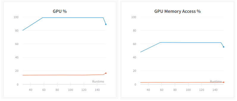

GPU % tracks the percent of the time over the past sample period during which one or more kernels was executing on the GPU.

Multiple GPUs

Next, let's see what will change when two GPUs are used. The picture below shows that the two GPUs have similar statistics on all four metrics. The GPU % graph indicates only 90% GPU utilizations on average. This is due to the overhead of parameter synchronization between two the devices. The overall training throughput is 6100 images/sec, which is also around 88% of the ideal throughput of running two GPUs independently (3500 x 2 = 7000). At the same time, the GPU Memory Access % is kept at 55%, indicating very small overhead of fetching data from memory.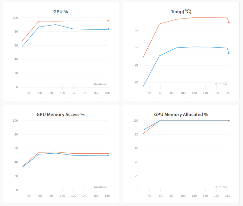

Real Data

So far we run training with synthetic data -- the images are generated on the GPU, and no augmentation (image distortion in spatial and color space) is used. To measure the performance on real data, we repeat the two-GPU training with pre-generated TFRecords of ImageNet and switch on the data augmentation. What we expect to see is the change in previously zero systems and IO utilization (CPU %, Memory % ad Disk), as well as the impact on the GPU utilization.

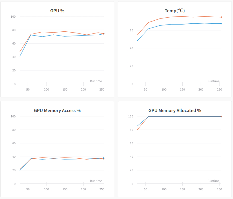
The immediate change is CPU %, which is now nearly 100%. This indicates that the data augmentation now becomes the bottleneck of the training. Memory % also increased to over 20%, but is still far from the limit, which indicates that system memory is unlikely to become the bottleneck of the training. Disk % also hardly changed, thanks to the efficient data format of TFRecord.

At the same time, we also observe a significant performance drop in GPU utilization: GPU % dropped to around 75%. In fact, the overall training throughput dropped to 4300 images/sec. This proves that the training throughput is indeed affected by the data augmentation that is running on the CPU.

Notice, AlexNet is a relatively light-weight network and thus the GPU computation is able to churn through a high number of images per second and thus cause the CPU to become bottlenecked. Some other networks, for example, ResNet152, have significantly more intense GPU computation and will not have this problem.

Summary

In this blog, we discuss how to use Weights and Biases for inspecting the efficiency of TensorFlow training jobs. In particular, the system section in wandb's dashboard tracks system utilization and gives you the insight of the computation/communication bottleneck. We think having a centralized place for bookkeeping your machine learning experiments is extremely valuable, and hope you think so too.

To learn more about wandb, check out their website: https://www.wandb.com.

We thank the wandb team, especially Lukas, Adrian, Carey, and Kenna for tutorials and help with my questions.