The problem
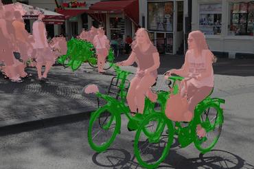
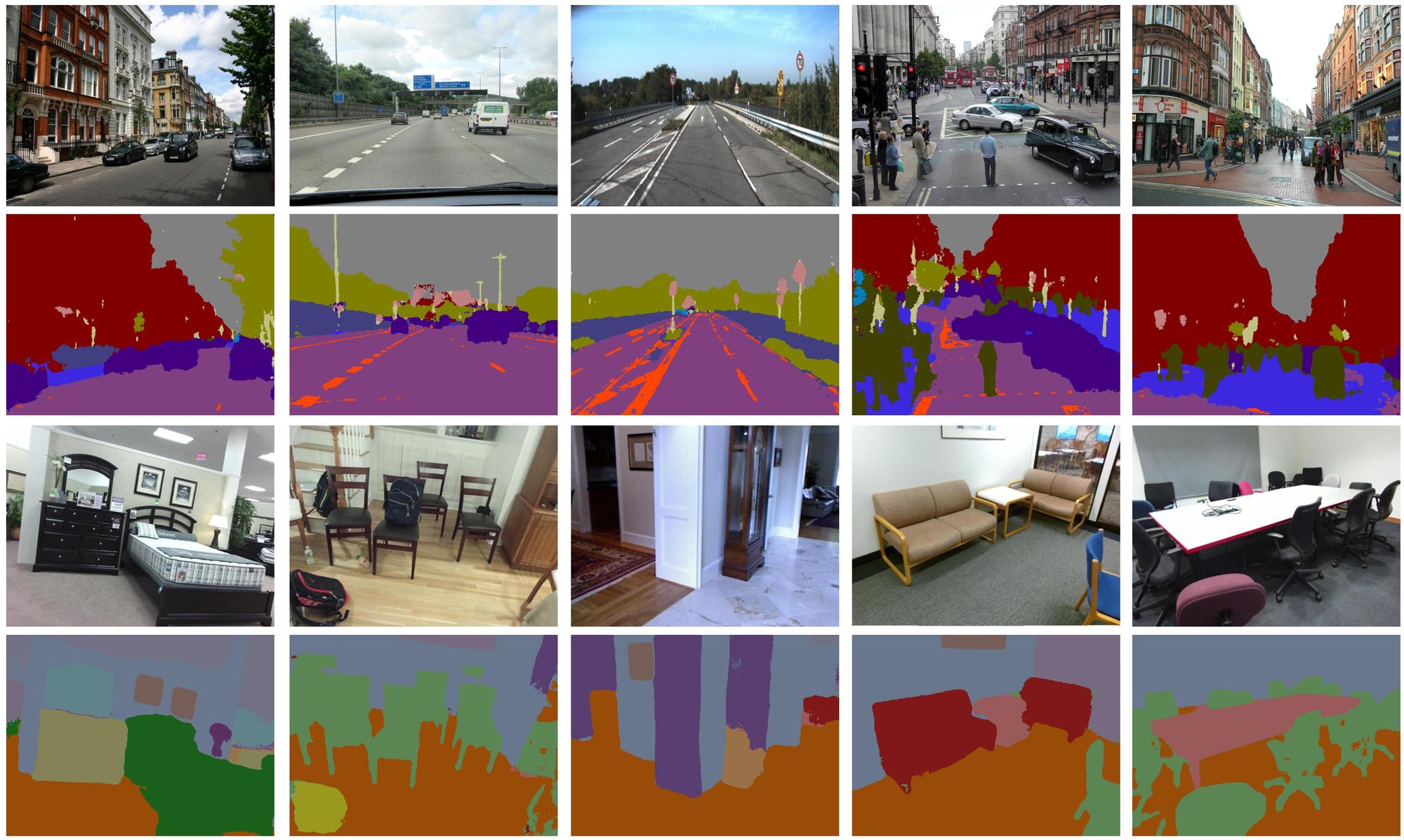
Image segmentation is the problem of assigning each pixel in an image a class label. Obviously, a single pixel doe not contain enough information for semantic understanding, and the decision should be made by putting the pixel in to a context (combining information from its local neighborhood).
The challenge of image segmentation is to come up with a mathematical model that does not only capture the uniqueness of individual pixels but also the interaction between adjacent pixels. For many years the state of the art model for this task is conditional random fields, or CRFs or short. It uses an unary term to penalize the miss classification of individual pixels, and a pairwise term to penalize the incoherent labeling between adjacent pixels, unless there is clear evidence for a boundary of object. Higher order term are also used to capture long-range dependencies. The downside is the terms need to be very carefully hand-crafted, and inference requires expensive computation.
On the other hand, convolutional neural networks (CNNs) has recently shown some very promising results in image segmentation. An important reason is the Markovian nature of CNNs that come with overlapped receptive fields and parameter sharing. This allows CNNs to be a simple but effective model that "learns" important features and the local interactions between these features for semantic segmentation.
In the rest of this tutorial, we will explain the main ideas behind some of the popular networks for image segmentation, including fully convolutional networks and U-Net.
| Network | FCN | U-Net |
|---|---|---|
| Training Speed (images/sec) | 185 | 160 |
| Accuracy | 86.6% | 86.9% |
| Total training time | 6.5 mins (200 epochs) | 7.5 mins (200 epochs) |
- Hardware: Lambda Single i7-7820X CPU + 1 x GeForce 1080 Ti
- OS: Ubuntu 18.04 LTS with Lambda Stack
You can jump to the code and the instructions from here.
Fully Convolutional Networks
Image segmentation can be viewed as a "dense classification" problem: we assign each pixel a class label. This requires the network to work with images of different sizes, different from a image classification network which only works with fixed size images due to the use of fully-connected layers.
Luckily, it is possible to adapt a classification network for segmentation tasks: simply replacing the fully connected layer by a ordinary convolution layer, so the network becomes fully convolutional and generates a "class heat map" instead of a "class vector". The implementation of this change can be as simple as this:
# Image classification
# A fully connected layer for image classification
inputs = tf.reshape(inputs, [batch_size, -1])
outputs = tf.layers.dense(inputs=inputs, units=num_classes)

# Image segmentation
# Change it to a convolutional layer for image segmentation
outputs = tf.layers.conv2d(inputs=inputs, filters=num_classes, kernel_size=[h, w])
Learning Up-sampling via Deconvolution
One caveat of the aforementioned approach is the reduction of image resolution. For example, a fully convolutional network adapted from VGG19 produces results that are downsized by a factor of 32, due to the use of five pooling layers. One might be tempted to use fewer pooling layers. However, doing so reduces the receptive field of the classifier and often leads to weaker performance and noisy outputs. One might consider scaling up the class heat map using bi-linear interpolation. However, it is unlikely to achieve accurate object localization with such a naive interpolation method.
Instead, it is better to use so called "deconvolution" to up-sample the output. We know down-sampling an image by a factor of S can be achieved by a convolution with stride of S. Similarly, up-sampling an image with factor of S can be achieved by a deconvolution with stride of S. Intuitively, a deconvolution "spray" a transposed filter onto the output feature map, and permits strides as an ordinary convolution does. If this sounds confusing, here is an interactive deconvolution demo to play around.
The advantage of deconvolution over naive interpolation (for example, bilinear or nearest neighbor) is it learns more useful interpolation rules based on semantic (as opposed to spatial distance between pixels). This allows the network to say "OK, since I saw this pattern in the low resolution input, the object must look like this in the higher resolution."
The FCN paper produces its best results by concatenating three feature maps from the down-sampling stage and up-sampling the concatenated result using a single deconvolution layer with stride of 8.
U-Net
The FCN architecture proposed an interesting idea: the input of each deconvolution layer is some concatenated feature maps from the down-sampling stage. This allows fine-grained details to be feed into the deconvolution process, as well as a more efficient gradient back-propagation to the early layers.
This idea has been further developed by researchers at University of Freiburg. Their U-Net expanded the up-sampling part of the network so it is almost symmetric to the down-sampling path, hence yields a u-shaped architecture. This equips the network with more "skip connections" and allows the optimal usage of these connections to be learned.
The implementation of such a U-Net is also straight forward. For example, this is a toy example that has only two down-sampling layers and two up-sampling layers:
encoder1 = tf.layers.conv2d(inputs=inputs,
                            filters=8,
                            kernel_size=[4, 4],
                            strides=(2, 2))
encoder2 = tf.layers.conv2d(inputs=encoder1,
                            filters=16,
                            kernel_size=[4, 4],
                            strides=(2, 2))
decoder2 = tf.layers.conv2d_transpose(inputs=encoder2,
                                      filters=8,
                                      kernel_size=[4, 4],
                                      strides=(2, 2))
# Concatenate feature map from the down-sampling path with the feature map from the up-sampling path. Assuming data format is channels_last
outputs = tf.concat([encoder1, decoder2], 3)
decoder1 = tf.layers.conv2d_transpose(inputs=outputs,
                                      filters=num_classes,
                                      kernel_size=[4, 4],
                                      strides=(2, 2))
Checkboard Artifact
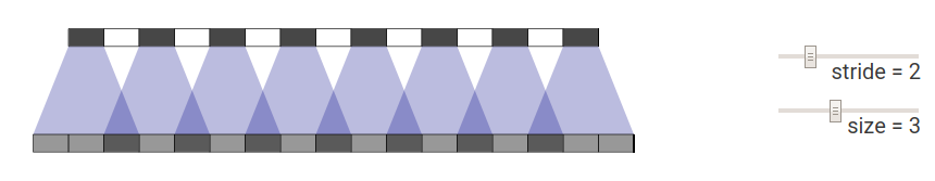
One common complaint people have about deconvolution is the checkerboard artifact. It is clearly illustrated in this study as the result of incompatible filter size and stride.
Roughly speaking, deconvolution spray the some "paint" (pattern encoded in the filter) onto a "canvas" (output feature map). The problem raises when the filter size is not divisible by the stride, which causes a periodic, uneven distribution of paint on the canvas. For example, this is what happens if the deconvolution uses filter size 3 and stride 2:
In contrast, use filter size 4 and stride 2 will not have this problem:
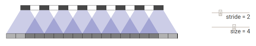
So one good practice for using deconvolution layer is to use filter size that is divisible by the stride. Besides, one can replace deconvolution by fractionally strided convolution, which can be implemented by first scaling up the input image using a simple interpolation algorithm (like nearest neighbor) with a factor of S, then apply regular convolution with a stride 1. This will effectively up-sample the image by a factor of S and avoid the checkerboard artifact.
Final Note
The type of architecture used in the U-Net has been widely studied by applications beyond image segmentation. In fact you might be more familiar with the term "auto-encoder", which has a contracting path and an expanding path that is more or less symmetric. Over the past few years the auto-encoder architecture has gained enormous success in the general task of image-to-image translation, including segmentation, depth estimation, super-resolution and stylization. This shows the image statistics learnt by a deep neural network is not only useful for compressing the information (encode) but also good at generative task (decode). We will see more of this in many of the other demos.
Demo
You can download the demo from this repo.
git clone https://github.com/lambdal/lambda-deep-learning-demo.git
You'll need a machine with at least one, but preferably multiple GPUs and you'll also want to install Lambda Stack which installs GPU-enabled TensorFlow in one line.
https://lambdalabs.com/lambda-stack-deep-learning-software
Once you have TensorFlow with GPU support, simply run the following the guidance on this page to reproduce the results.