Our last tutorial described how to do basic image classification with TensorFlow. In this tutorial, we will demonstrate how to use a pre-trained model for transfer learning. The networks used in this tutorial include ResNet50, InceptionV4 and NasNet. The dataset is Stanford Dogs.
| Network | ResNet50 | InceptionV4 | NasNet-A-large |
|---|---|---|---|
| Training Speed (images/sec) | 770 | 315 | 128 |
| Top-1 Accuracy | 76.6% | 93.1% | 95.2% |
| Total training time | 155 secs (10 epochs) | 76 secs (2 epochs) | 182 secs (2 epochs) |
- Hardware: Lambda Quad i7-7820X CPU + 4x GeForce 1080 Ti
- OS: Ubuntu 18.04 LTS with Lambda Stack
You can jump to the code and the instructions from here.
The Goal
There was a time when handcrafted features and models just worked a lot better than artificial neural networks. This was changed by the popularity of GPU computing, the birth of ImageNet, and continued progress in the underlying research behind training deep neural networks. We have seen the birth of AlexNet, VGGNet, GoogLeNet and eventually the super-human performance of A.I. in object recognition.
However, the success of deep neural networks also raises an important question: How much data is enough for training these models? Ideally, we'd prefer to minimize efforts in data collection, labeling, and cleaning. One approach that is currently used to reduce the burden of data collection and labeling is transfer learning. Transfer learning is adapting a model trained for one purpose to be used for another. In this case, adapting a model trained on ImageNet to work with a smaller dataset of your own. The main hypothesis which allows transfer learning to work is:
Features learned from on a large dataset should generalize to new tasks.
Transfer learning works surprisingly well for many problems, thanks to the features learned by deep neural networks. The rest of this tutorial will cover the basic methodology of transfer learning, and showcase some results in the context of image classification.
The Method
Transfer learning is a straightforward two-step process:
- Initialize the model with weights from a pre-trained model;
- Train the model on the new data.
What is less straightforward is deciding how much deviation from the first trained model we should allow. This is important because we need to strike a balance between the prior knowledge learned from the large dataset and the potential new knowledge that can be gained from the new dataset.
At one end of the spectrum, one can be conservative and freeze all but the last layer of the network. In this way, the pre-trained model acts as a "feature extractor" and the second training step only acts to re-learn the fully connected layers to classify those features differently. This is useful when the new dataset is closely related to the old dataset, in which case the pre-trained model offers highly relevant features to the new task. The fact that many of the weights are not trainable also means faster training speed and robustness to over-fitting. Preventing over-fitting is particularly important when the new dataset is small. Because, as the dataset decreases in size, you reduce your ability to constrain a large number of parameters. Remember: as the model capacity (number of parameters) increases, you'll need more data to constrain those parameters.
At the other end of the spectrum, we can be aggressive and allow all of the layers to remain trainable. In this instance, the pre-trained model acts as a "weights initializer" and the training affects all layers. This is better when the new dataset and the old dataset are not closely related, or, the new dataset has more data than the old dataset. The benefit is that you allow the training algorithm to explore a higher dimensional complex parameter space and hopefully find a parameter set with lower error. However, the downside is that with more free parameters in the model, training will be slower and you'll have a higher risk of over-fitting. As John Von Neumann famously said:
With four parameters I can fit an elephant, and with five I can make him wiggle his trunk.
We can choose a balanced strategy by making a few layers trainable (as opposed to making all layers or only a single layer trainable). We recommend Yosinski, Clune, et al. 2014 to readers who are interested in learning more about tuning the layers for transfer learning.
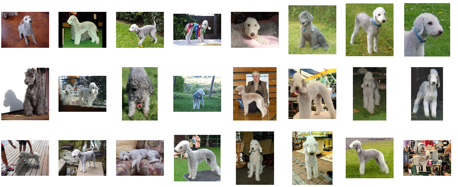
The rest of this tutorial will show how to use transfer learning to classify dog breeds. We will use a few classic networks as the pre-trained models, including ResNet50, InceptionV4 and NasNet-A-Large. The new dataset we use is the Stanford Dogs dataset, which has in total 20,580 images of 120 different breeds of dogs. Because these dog classes are closely related to (in fact, a subset of) the ImageNet, we choose the feature extractor approach which is fast to train and has lower risk of overfitting.
Let's dive in!
Demo
You can download the demo from this repo.
git clone https://github.com/lambdal/lambda-deep-learning-demo.git
You'll need a machine with at least one, but preferably multiple GPUs and you'll also want to install Lambda Stack which installs GPU-enabled TensorFlow in one line.
https://lambdalabs.com/lambda-stack-deep-learning-software
Once you have TensorFlow with GPU support, simply run the following the guidance on this page to reproduce the results.
Additional Notes:
Below, we'll dive into some implementation details. Let's use ResNet50 as an example.
Create the network: The following TensorFlow code creates a ResNet50 Network for 120 classes (the number of classes in Stanford Dogs dataset):
inputs = A tensor of [batch_size, height, width, channel] # image data
num_classes = 120 # Number of output classes
is_training = True # Set to False for evaluation and inference

# TF-slim's arg_scope defines default settings for specific operations.
with slim.arg_scope(resnet_v2.resnet_arg_scope()):
    # Create ResNet50
    logits, _ = resnet_v2.resnet_v2_50(inputs,
                                       num_classes,
                                       is_training=is_training)
The output logits is a tensor of shape [batch_size, num_classes]. You can think each row in this tensor as a 120-dimensional vector for the class scores of an image.
A quick aside on Batch Normalization: Notice the is_training flag is needed by a particular type of layer called batch normalization, or batch norm for short. A batch normalization layer acts differently depending on whether you are training or testing. During training, batch norm normalizes the output of the previous layer based on the statistics (mean / variance) of the batch. During testing or inference, the normalization layer normalizes based on global statistics calculated with a moving average that is built up during training time. You can find more details about batch normalization from reading the very approachable original Batch Normalization paper or from this Coursera course. In short, if your network has a batch normalization layer, be sure to properly set the training mode. This applies regardless of which framework you're using.
Restore weights: after created the model, we initialize its weights from a pre-trained model:
# Set the path to the pre-trained model
pretrained_model = path_to_pre-trained_model

# Get all variables from the model.
variables_to_restore = {v.name.split(":")[0]: v
                        for v in tf.get_collection(
                            tf.GraphKeys.GLOBAL_VARIABLES)}

# Skip some variables during restore.
skip_pretrained_var = ["resnet_v2_50/logits", "global_step"]
variables_to_restore = {
    v: variables_to_restore[v] for
    v in variables_to_restore if not
    any(x in v for x in skip_pretrained_var)}

# Restore the remaining variables
if variables_to_restore:
  saver_pre_trained = tf.train.Saver(
    var_list=variables_to_restore)

  saver_pre_trained.restore(sess, pretrained_model)
Caveats
- We use
GLOBAL_VARIABLESto restore not only the trainable variables but also the non-trainable variables (as opposed to usingTRAINABLE_VARIABLESwhich only includes the trainable). This is because we want to restore the moving statistics for batch normalization layers so these statistics can converge faster in (in comparison to randomly initialize these statistics). - We use the
skip_pretrained_varlist to skip some variables during restoration, including the weights from the last layer (resnet_v2_50/logits) and the number of steps are used in producing the pre-trained modelglobal_step. We do not need them in transfer learning. - This restoration process should happen after the creation of the network and before the training. Our demo suite implement it inside the
before_runmember function of basic callback class.
Training with New Data: Now that we have created a ResNet50 with weights restored from the pre-trained model, we need to train the network on the new dataset. In particular, we use the trainable_var list to select the trainable variables. In this case all layers are frozen except for the ones whose name prefixed by "resnet_v2_50/logits".
# Collect all trainale variables
train_vars = tf.get_collection(
  tf.GraphKeys.TRAINABLE_VARIABLES)

# Discard variables that are not in the last layer
trainable_var = ["resnet_v2_50/logits"]

train_vars = [v for v in train_vars
              if any(x in v.name
                     for x in
                     trainable_vars)]

# Performs gradient decent on the trainable variables
optimizer = tf.train.MomentumOptimizer(learning_rate=0.1, momentum=0.9)
grads = optimizer.compute_gradients(loss, var_list=train_vars)
minimize_op = optimizer.apply_gradients(grads)
That's it. The key steps are specifying the filters for selecting which layers we will modify in the transfer learning (in skip_pretrained_var and train_vars). In this feature extractor example, the variables to train happens to be the variables to skip at restoration. Generally speaking, you can switch between the feature extractor approach and the fine-tune-all-layers approach with different settings of these filters.