This tutorial shows you how to perform transfer learning using TensorFlow 2.0. We will cover:
- Handling customized datasets
- Restoring backbone network with Keras's application API
- Restoring backbone network from disk
Reproduce the tutorial
All code in this tutorial can be found in this repository.
python download_data.py \
--data_url=https://s3-us-west-2.amazonaws.com/lambdalabs-files/StanfordDogs120.tar.gz \
--data_dir=~/demo/data

python transfer_dogs.py
Customized Data
In this tutorial, we will classify images in the Stanford Dogs dataset. We re-organized the raw data with a CSV file. The first column is the path to the image, the second column is the class id. The csv file is placed in ~/demo/data/StanfordDogs120/train.csv. (This will change if you modify the --data_dir parameter.)
We first load the csv files into a list of path to the images and a list of of labels:
def load_csv(file):
  dirname = os.path.dirname(file)
  images_path = []
  labels = []
  with open(file) as f:
    parsed = csv.reader(f, delimiter=",", quotechar="'")
    for row in parsed:
      images_path.append(os.path.join(dirname, row[0]))
      labels.append(int(row[1]))
  return images_path, labels

TRAIN_FILE = path_home + "/demo/data/StanfordDogs120/train.csv"
train_images_path, train_labels = load_csv(TRAIN_FILE)
Next we create a TensorFlow Dataset from these list:
train_dataset = tf.data.Dataset.from_tensor_slices((train_images_path, train_labels))
Here's the pre-processing pipeline:
- Read the images from their paths.
- Since the sizes of the images are not standard, we resize them so they can be batch pre-processed. It is important to preserve the aspect ratio of each image during resizing. Otherwise, the objects (dogs in this case) will be distorted. In our experiment, distortion caused over 10% reduction of testing accuracy.
- We augment the data by resizing each image randomly to a width uniformly selected from a distribution between
[256, 512]then randomly crop a 224x224 sub-image out of it. During testing, we resize the image, so its width is 256, and then centr crop a 224x224 sub-image. - During training, we perform random horizontal flipping.
- We subtract ImageNet's mean RGB value from all images.
HEIGHT = 224
WIDTH = 224
RESIZE_SIDE_MIN = 256
RESIZE_SIDE_MAX = 512
R_MEAN = 123.68
G_MEAN = 116.78
B_MEAN = 103.94

def preprocess_for_train(x, y):
    x = tf.compat.v1.read_file(x)
    x = tf.image.decode_jpeg(x, dct_method="INTEGER_ACCURATE")
    resize_side = tf.random.uniform(
        [], minval=RESIZE_SIDE_MIN, maxval=RESIZE_SIDE_MAX + 1, dtype=tf.int32)
    x = _aspect_preserving_resize(x, resize_side)
    x = _random_crop([image], HEIGHT, WIDTH)[0]
    x.set_shape([HEIGHT, WIDTH, 3])
    x = tf.cast(x, tf.float32)
    x = tf.image.random_flip_left_right(image)
    x = _mean_image_subtraction(x, [R_MEAN, G_MEAN, B_MEAN])
  return x, y

def preprocess_for_eval(x, y):
    x = tf.compat.v1.read_file(x)
    x = tf.image.decode_jpeg(x, dct_method="INTEGER_ACCURATE")
    x = _aspect_preserving_resize(x, RESIZE_SIDE_MIN)
    x = _central_crop([x], HEIGHT, WIDTH)[0]
    x.set_shape([HEIGHT, WIDTH, 3])
    x = tf.cast(x, tf.float32)
    x = _mean_image_subtraction(image, [R_MEAN, G_MEAN, B_MEAN])
  return x, y
The customized resizing functions are implemented in this script. Notice the shuffle function is applied first. This means the shuffling is applied to the paths of the images, which is significantly faster than applying to the images themselves.
NUM_TRAIN_SAMPLES = len(train_images_path)
train_dataset.shuffle(NUM_TRAIN_SAMPLES).map(preprocess_for_train).map(augmentation).batch(BS_PER_GPU, drop_remainder=True)
test_dataset = test_dataset.map(preprocess_eval).batch(BS_PER_GPU, drop_remainder=True)
We can now sample from this dataset:
for image, label in train_dataset.take(1):
  print(image.shape, label.shape)

(batch_size, 224, 224, 3) (batch_size,)
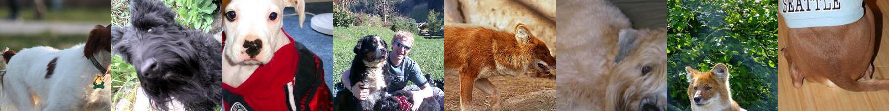
These are samples of the images generated by the training dataset:
Restore Backbone Network (Keras applications)
Keras pakage a number of deep leanring models alongside pre-trained weights into an applications module. These models can be used for transfer learning. To create a model with weights restored:
backbone = tf.keras.applications.ResNet50(weights = "imagenet", include_top=False)
backbone.trainable = False
Set weights = "imagenet" to restore weights trained with ImageNet. Set include_top=False to skip the top layer during restoration. Remember to set trainable to False to freeze the weights during training. Freezing the backbone model weights is useful when the new dataset is significantly smaller than the original dataset used to train the backbone model. By freezing the pre-trained weights, the model is less likely to over-fit.
Next, we add append a few layers to the backbone. The first one is a GlobalAveragePooling2D layer, which takes the output of the backbone as the input. This layer computes the per-channel mean of the feature map, an operation that is spatially invariant. Then, a dropout layer is applied to improve the generalization performance. Finally, a fully connected layer with a softmax outputs a categorical probability distribution across.
x = tf.keras.layers.GlobalAveragePooling2D(name='avg_pool')(x)
x = tf.keras.layers.Dropout(0.5)(x)
x = tf.keras.layers.Dense(NUM_CLASSES, activation='softmax',
                          name='prediction')(x)
model = tf.keras.models.Model(backbone.input, x, name='model')
To train this model, we simply compile() and fit() it using the dataset we created previously.
NUM_EPOCHS = 10
opt = tf.keras.optimizers.SGD()
model.compile(optimizer=opt,
        loss='sparse_categorical_crossentropy',
        metrics=['accuracy'])
model.fit(train_dataset,
          epochs=NUM_EPOCHS,
          validation_data=test_dataset,
          validation_freq=1,
          callbacks=[tensorboard_callback, lr_schedule_callback])
The learning rate schedule generates a step function that decays the initial learning rate (0.1) by a factor of 10 at the 6th and 9th epochs. After ten epochs of training, this network achieves a 75% testing accuracy.
Restore Backbone (from disk)
In case the backbone model is not included in the Keras applications module, one can also restore it from the disk through a .h5 file (which follows the HDF5 specification).
To demonstrate this, we restore the ResNet50 using the Keras applications module, save it on disk as an .h5 file, and restore it as a backbone.
model = tf.keras.applications.ResNet50(weights = "imagenet", include_top=True)
model.save('ResNet50.h5')
backbone = tf.keras.models.load_model('ResNet50.h5')
backbone.trainable = False
To append new layers to the backbone, one needs to specify the input layers. In this case, it is the third to last layer that is used:
x = backbone.layers[-3].output
x = tf.keras.layers.GlobalAveragePooling2D(name='avg_pool')(x)
...
model = tf.keras.models.Model(backbone.input, x, name='model')
This model can be trained in the same way as the previous one whose backbone was restored as a Keras application.
Summary
In this tutorial, we explained how to perform transfer learning in TensorFlow 2. The key is to restore the backbone from a pre-trained model and add your own custom layers. To this end, we demonstrated two paths: restore the backbone as a Keras application and restore the backbone from a .h5 file. The latter is more general as it can be used to deal with customized models that are not included in Keras applications.
We also showed how to add new layers to the backbone and implement customized data pipeline.
All code in this tutorial can be found in this repo.