The problem
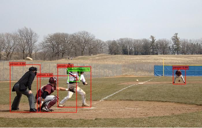
The task of object detection is to identify "what" objects are inside of an image and "where" they are. Given an input image, the algorithm outputs a list of objects, each associated with a class label and location (usually in the form of bounding box coordinates). In practice, only limited types of objects of interests are considered and the rest of the image should be recognized as object-less background.
Object detection has been a central problem in computer vision and pattern recognition. It does not only inherit the major challenges from image classification, such as robustness to noise, transformations, occlusions etc but also introduces new challenges, for example, detecting multiple instances, identifying their precise locations in the image etc.
Before the renaissance of neural networks, the best detection methods combined robust low-level features (SIFT, HOG etc) and compositional model that is elastic to object deformation. A classic example is "Deformable Parts Model (DPM) ", which represents the state of the art object detection around 2010. However, its performance is still distanced from what is applicable in real-world applications in term of both speed and accuracy. Moreover, these handcrafted features and models are difficult to generalize – for example, DPM may use different compositional templates for different object classes.
Since the 2010s, the field of object detection has also made significant progress with the help of deep neural networks. In this tutorial we demonstrate one of the landmark modern object detectors – the "Single Shot Detector (SSD)" invented by Wei Liu et al.
| Network | SSD300 | SSD512 |
|---|---|---|
| Training Speed (images/sec) | 145 | 65 |
| (AP) IoU=0.50:0.95, area=all, maxDets=100 | 21.9 | 25.7 |
| Total training time (100 epochs) | 23.5 hours | 42.5 hours |
- Hardware: Lambda Quad i7-7820X CPU + 4 x GeForce 1080 Ti
- OS: Ubuntu 18.04 LTS with Lambda Stack
You can jump to the code and the instructions from here.
Single-Shot Detector
Let's first remind ourselves about the two main tasks in object detection: identify what objects in the image (classification) and where they are (localization). In essence, SSD is a multi-scale sliding window detector that leverages deep CNNs for both these tasks.
A sliding window detection, as its name suggests, slides a local window across the image and identifies at each location whether the window contains any object of interests or not. Multi-scale increases the robustness of the detection by considering windows of different sizes. Such a brute force strategy can be unreliable and expensive: successful detection requests the right information being sampled from the image, which usually means a fine-grained resolution to slide the window and testing a large cardinality of local windows at each location.
SSD makes the detection drastically more robust to how information is sampled from the underlying image. Let's first summarize the rationale with a few high-level observations:
- Deep convolutional neural networks can classify object very robustly against spatial transformation, due to the cascade of pooling operations and non-linear activation. This is something well-known to image classification literature and also what SSD is heavily leveraged on. In essence, SSD does sliding window detection where the receptive field acts as the local search window. Just like all other sliding window methods, SSD's search also has a finite resolution, decided by the stride of the convolution and the pooling operation. It will inevitably get poorly sampled information – where the receptive field is off the target. Nonetheless, thanks to deep features, this doesn't break SSD's classification performance – a dog is still a dog, even when SSD only sees part of it!
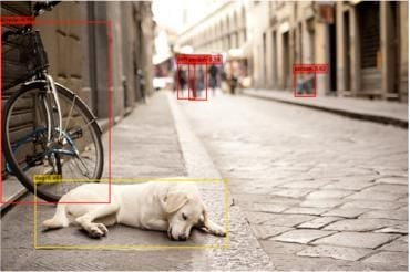
- Deep convolutional neural networks can predict not only an object's class but also its precise location. Precisely, instead of mapping a bunch of pixels to a vector of class scores, SSD can also map the same pixels to a vector of four floating numbers, representing the bounding box. This is very important. The detection is now free from prescripted shapes, hence achieves much more accurate localization with far less computation. This is something pre-deep learning object detectors (in particular DPM) had vaguely touched on but unable to crack.
- Last but not least, SSD allows feature sharing between the classification task and the localization task. In fact, only the very last layer is different between these two tasks. This significantly reduced the computation cost and allows the network to learn features that also generalize better.
While the concept of SSD is easy to grasp, the realization comes with a lot of details and decisions. Next, let's discuss the implementation details we found crucial to SSD's performance.
Implementation Details
Input and Output: The input of SSD is an image of fixed size, for example, 512x512 for SSD512. The fixed size constraint is mainly for efficient training with batched data. Being fully convolutional, the network can run inference on images of different sizes.
The output of SSD is a prediction map. Each location in this map stores classes confidence and bounding box information as if there is indeed an object of interests at every location. Obviously, there will be a lot of false alarms, so a further process is used to select a list of most likely prediction based on simple heuristics.
To train the network, one needs to compare the ground truth (a list of objects) against the prediction map. This is achieved with the help of priorbox, which we will cover in details later.
Multi-scale Detection: The resolution of the detection equals the size of its prediction map. Multi-scale detection is achieved by generating prediction maps of different resolutions. For example, SSD512 outputs seven prediction maps of resolutions 64x64, 32x32, 16x16, 8x8, 4x4, 2x2, and 1x1 respectively. You can think there are 5461 "local prediction" behind the scene. The input of each prediction is effectively the receptive field of the output feature.
Priorbox: Heads up – this is important!
We know the ground truth for object detection comes in as a list of objects, whereas the output of SSD is a prediction map. We also know in order to compute a training loss, this ground truth list needs to be compared against the predictions. The question is, how?
- There can be multiple objects in the image. In this case which one or ones should be picked as the ground truth for each prediction?
- There can be locations in the image that contains no objects. How to set the ground truth at these locations?
Intuitively, object detection is a local task: what is in the top left corner of an image is usually unrelated to predict an object in the bottom right corner of the image. So one needs to measure how relevance each ground truth is to each prediction, probably based on some distance based metric.
This is where priorbox comes into play. You can think it as the expected bounding box prediction – the average shape of objects at a certain scale. We can use priorbox to select the ground truth for each prediction. This is how:
- We put one priorbox at each location in the prediction map.
- We compute the intersect over union (IoU) between the priorbox and the ground truth.
- The ground truth object that has the highest IoU is used as the target for each prediction, given its IoU is higher than a threshold.
- For predictions who have no valid match, the target class is set to the background class and they will not be used for calculating the localization loss.
Basically, if there is significant overlapping between a priorbox and a ground truth object, then the ground truth can be used at that location. The class of the ground truth is directly used to compute the classification loss; whereas the offset between the ground truth bounding box and the priorbox is used to compute the location loss.
More on Priorbox: The size of the priorbox decides how "local" the detector is. Smaller priorbox makes the detector behave more locally, because it makes distanced ground truth objects irrelevant. It is good practice to use different sizes for predictions at different scales. For example, SSD512 uses 20.48, 51.2, 133.12, 215.04, 296.96, 378.88 and 460.8 as the sizes of the priorbox at its seven different prediction layers. The details for computing these numbers can be found here.
In practice, SSD uses a few different types of priorbox, each with a different scale or aspect ratio, in a single layer. Doing so creates different "experts" for detecting objects of different shapes. For example, SSD512 use 4, 6, 6, 6, 6, 4, 4 types of different priorboxes for its seven prediction layers, whereas the aspect ratio of these priorboxes can be chosen from 1:3, 1:2, 1:1, 2:1 or 3:1. Notice, experts in the same layer take the same underlying input (the same receptive field). They behave differently because they use different parameters (convolutional filters) and use different ground truth fetch by different priorboxes.
Hard negative mining: Priorbox uses a simple distance-based heuristic to create ground truth predictions, including backgrounds where no matched object can be found. However, there can be an imbalance between foreground samples and background samples, as background samples are considerably easy to obtain. In consequence, the detector may produce many false negatives due to the lack of a training signal of foreground objects.
To address this problem, SSD uses hard negative mining: all background samples are sorted by their predicted background scores in the ascending order. Only the top K samples are kept for proceeding to the computation of the loss. K is computed on the fly for each batch to keep a 1:3 ratio between foreground samples and background samples.
Data augmentation: SSD use a number of augmentation strategies. A "zoom in" strategy is used to improve the performance on detecting large objects: a random sub-region is selected from the image and scaled to the standard size (for example, 512x512 for SSD512) before being fed to the network for training. This creates extra examples of large objects. Likewise, a "zoom out" strategy is used to improve the performance on detecting small objects: an empty canvas (up to 4 times the size of the original image) is created. The original image is then randomly pasted onto the canvas. After which the canvas is scaled to the standard size before being fed to the network for training. This creates extras examples of small objects and is crucial to SSD's performance on MSCOCO.
Pre-trained Feature Extractor and L2 normalization: Although it is possible to use other pre-trained feature extractors, the original SSD paper reported their results with VGG_16. There is, however, a few modifications on the VGG_16: parameters are subsampled from fc6 and fc7, dilation of 6 is applied on fc6 for a larger receptive field. It is also important to add apply a per-channel L2 normalization to the output of the conv4_3 layer, where the normalization variables are also trainable.
Post-processing: Last but not least, the prediction map cannot be directly used as detection results. For SSD512, there are in fact 64x64x4 + 32x32x6 + 16x16x6 + 8x8x6 + 4x4x6 + 2x2x4 + 1x1x4 = 24564 predictions in a single input image. SSD uses some simple heuristics to filter out most of the predictions: It first discards weak detection with a threshold on confidence score, then performs a per-class non-maximum suppression, and curates results from all classes before selecting the top 200 detections as the final output. To compute mAP, one may use a low threshold on confidence score (like 0.01) to obtain high recall. For a real-world application, one might use a higher threshold (like 0.5) to only retain the very confident detection.
Demo
You can download the demo from this repo.
git clone https://github.com/lambdal/lambda-deep-learning-demo.git
Follow the instructions in this document to reproduce the results.
You'll need a machine with at least one, but preferably multiple GPUs and you'll also want to install Lambda Stack which installs GPU-enabled TensorFlow in one line.
https://lambdalabs.com/lambda-stack-deep-learning-software
Once you have TensorFlow with GPU support, simply run the following the guidance on this page to reproduce the results.